I’m more and more intrigued by the potential spatial data hold for political science. Once you begin to think about it, concepts like proximity and clustering are basic building blocks for explaining social phenomena. Even better, since the idea of open data has gone mainstream, more and more spatially referenced information becomes available, and when it comes to free, open source software, we are spoilt for choice or, at least in my case, up and beyond the point of utter confusion.
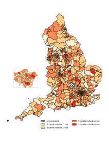
For our paper on the effect of spatial distance between candidates and their prospective voters, we needed a choropleth map of English Westminster constituencies that shows how many of the mainstream candidates live within the constituency’s boundaries. Basically, we had three options (not counting the rather few user-contributed packages for Stata): GRASS, a motley collection of Python packages, and a host of libraries for R.
GRASS is a full-blown open source GIS, whose user interface is perfect for keyboard aficionados and brings back happy memories of the 1980s. While GRASS can do amazing things with raster and vector maps, it is suboptimal for dealing with rectangular data. In the end, we used only its underrated cartographic ps.map module, which reliably creates high-resolution postscript maps.
Python has huge potential for social scientists, both in its own right and as a kind of glue that binds various programs together. In principle, a lot of GIS-related tasks could be done with Python alone. We used the very useful geopy toolboxfor converting UK postcodes to LatLong co-ordinates, with a few lines of code and a little help from Google.

The real treasure trove, however, is R. The quality of packages for spatial analysis is amazing, and their scope is a little overwhelming. Applied Spatial Data Analysis with R by Roger Bivand, who wrote much of the relevant code, provides much-needed guidance.
Counting the number of mainstream candidates living in a constituency is a point-in-polygon problem: each candidate is a co-ordinate enclosed by a constituency boundary. Function overlay from package sp carries out the relevant operation. Once I had it located, I was seriously tempted to loop over constituencies and candidates. Just in time, I remembered the R mantra of vectorisation. Provided that points (candidates) and polygons (constituencies) have been transformed to the same projection, all that is needed is this:
 mymap@data$homeconst1 <-overlay(candpos1,mymap)
 mymap@data$homeconst2 <-overlay(candpos2,mymap)
 mymap@data$homeconst3 <-overlay(candpos3,mymap)
This works because candpos1 is a vector of points that represent the spatial positions of all Labour candidates. These are tested against all constituency boundaries. The result is another vector of indices, i.e. sequence numbers of the constituencies the candidates are living in. Put differently, overlay takes a list of points and a bunch of polygons and returns a list that maps the former to the latter. With a bit of boolean logic, a vector of zeros (candidate outside constituency) and ones (candidate living in their constituency) ensues. Summing up the respective vectors for Labour, Tories, and LibDems then gives the required count that can be mapped. Result!

Discover more from kai arzheimer
Subscribe to get the latest posts sent to your email.

Nice. I can imagine myself spending ages writing a slow loop to do this and only finding out too late!
@chrishanretty That’s exactly what I did!